Semi-Supervised Hashing for Scalable Image Retrieval

In this paper, they propose the semi-supervised hashing method. This method solve the problem that unsupervised hashing methods doesn't consider the label of training data, and solve the problem that supervised hashing methods might be over-fitting when training data is small.

They first describe some hashing methods, including LSH, SH, and RBM.

●Locality Sensitive Hashing (LSH)

The main concept of LSH is to map similar samples to the same bucket with higher probability.

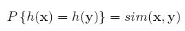
This probability can be implemented by random projection.

The following is the function of random projection.

The final hash code is created by concatenating multiple values of random projection functions.

In order to reduce the size of each bucket, K should be large enough.

However, it will also decrease the probability that similar samples fall in the same bucket.

Therefore, we need to use multiple hash tables, and it is inefficient.

●Spectral Hashing (SH)

Because of the inefficiency of random projection, SH appears.

SH try to minimize the following function.

where , k = 1...K

Optimizing this formula is NP-hard, thus it needs to be relaxed.

After relaxing the constraints, the optimization can be solved by spectral graph analysis.

I think that is why it is named "Spectral Hashing".

●Restricted Boltzmann Machines (RBMs)

This method try to learn belief networks by Restricted Boltzmann Machines.

RBMs has two critical stages: unsupervised pre-training and supervised fine-tuning.

The weakness of this method is that it needs to learn lots of weight.

For example, five layers of size 512-512-256-32 modes require to learn 663552 weights.

Therefore, it takes a long time to train.

After introducing three methods, all of them having weakness, they propose their method, semi-supervised hashing.

Let M denote the set of neighbor-pairs, and C denotes the set of nonneighbor-pairs.

Using the information of labeled data, the objective function is try to maximize the following function

Function h_k will only output 1 or -1. Thus, above function try to make the hash codes of neighbor-pairs to be the same, and make the codes of nonneighbor-pairs to be different.

This formula can be rewritten as a matrix format

Let S belong to R^(L*L), we can create the matrix by assigning the following values to each element

And the function becomes

W is the projection planes we want to learn

However, simply maximize this function is almost the same as supervised methods, and it will suffer form over-fitting. Thus, they add the regularization term.

They try to make every single bit hash function outputs the same number of "1" and "-1". That is, maximize the variance of each bit.

This optimization function is also NP-hard to solve again, so they relax the constraint next to solve it. I won't describe the solution details here. If you want to find how to solve it, please read the original paper.

The following is one of it experiments result.

We can find that SSH outperform other methods.

That is the same for the other dataset (gist dataset).

========================================================

Comment:

In this paper, they propose a method between the supervised and unsupervised method. That is a quite smart way to improve the performance. Like most of the thing, best case is often not happened at the extreme points. They often happened in the middle of extreme points. It tells us to think does there exist another problems that are not solved by using the method in the middle of the cases. Then, that might be a good choice for research.

Online Dictionary Learning for Sparse Coding

We know that sparse coding is one of the most used methods to quantize the features.

And the performance of sparse coding is highly related to the codebook (centroids) it uses.

Therefore, this paper want to provide a efficient method to learn the codebook well.

They said there are three main contributions in this paper

●Cast the dictionary learning problem into optimization problem, which minimizes the expected cost

●Propose a online learning algorithm

●The algorithm is significantly faster than previous algorithms

Before introducing their algorithm, let us first introduce the problem definition of sparse coding.

Given a set of signals X= [X1, ..., Xn], it want to minimize

where D is the learned dictionary (codebook). l is a function to measure the distance between original signal and quantized signal. That is, the quantization error. We not only want to minimize this function, but also want quantized signals to be sparse.Thus, there is a L1 term in the l function

Here we want to minimize the value of alpha. However, we can arbitrarily increase the elements in D to decrease the value of alpha. Thus, we have to constrain the value of elements in D.

The L2-norm of each column in D should be less than 1.

Finally, the problem becomes that

We need to solve two items in this equation. One is D, and the other is alpha.

It is quite hard to solve these two variables at the same. Therefore, we often solve one variable first by fixing another variable, and then solve another iteratively.

The following is the main algorithm of this paper

As we can see, it first solve alpha by using the D in previous iteration, and then solve D by fixing the alpha.

But learning a new dictionary for every input signal Xi is not efficient.

Instead, they train a new dictionary after collecting Eta signals, and using different updating methods as follow.

Experiments:

They compared the results of this online method with Batch method and the Stochastic Gradient Descent.

Objective function is fn(D),which is also known as quantization error. Thus, the smaller is the better.

We can found that the performance of online-learning is better than batch methods, and is almost the same as Stochastic Gradient Descent.

Although the performance is almost the same, Stochastic Gradient Descent needs to tune the learning rate Rho.

========================================================

Comment:

This paper describes a useful online codebook learning method. Although it has the term "Sparse Coding" in the title, it doesn't focus on this. It main focus on "Online learning".

They provide a very detail theoretical prove to convince the readers it is not just an ad-hoc method. That is quite important in this paper, but hard to read.

Furthermore, they said they have three contributions, but I think the first one is not the contribution from them.

Aggregating local descriptors into a compact image representation

In this paper, they focus on the large-scale image retrieval, and want two fulfill three factors at the same time: the search accuracy, its efficiency and the memory usage.

In order to fulfill these three factor, they proposed a new features representation method, VLAD (vector of locally aggregated descriptors). It can obtain a significantly higher accuracy with about 20-byte representation.

The other contribution of this paper is jointly optimizing the dimensional reduction and the indexation algorithm. Not like previous works, they often consider these two factors separately.

Thus, I will focus on these two things in the following.

●VLAD: vector of locally aggregated descriptors

The concept of VLAD is derive from BOF (Bof of features) and Fisher kernel.

They first learn a codebook C = {c1 , ..., ck } of k visual words with k-means.

Each local descriptor x is assigned to its nearest visual word ci = NN(x).

The idea of the VLAD descriptor is to accumulate, for each visual word ci, the differences x−ci of the vectors x assigned to ci.

Write the above things as the mathematical equation.

where x_j and c_i, j are the j-th component of x and ci

The following are the visual representation of the features and their images.

Each grid represent one centroid, and each point in the grid has 8 directions (like the representation as SIFT).

Thus, every centroid is a 16*8 = 128 dimension vector.

You can find that the images having similar visual contents tend to have the similar differences with centroids. So aggregating them together is reasonable.

●Converting vectors to codes

In this paper, they use the asymmetric distance computation (ADC), which only encodes the vectors of the database, but not the query vector.

For every features in the database, they first use PCA to do dimension reduction. The number of dimensions will reduce from D to D'. That is, we can find a D'×D matrix M such that the original feature x is transformed to x' = Mx.

After doing this, split x' into m subvectors, and quantized each subvector separately.

Centroids in each subvetors are computed separately by k-means.

The following is the presentation slide from the author. (he use y to represent x')

For every subvectors, they use the same number of centroids. However, after PCA, the variance of the different components of x′ is not balanced. The variance of first principle component tends to be much larger than the last one. Thus, using the same number of centroids will introduce more quantization error for first principle component.

To solve this problem, they try to find another transformation matrix Q, such that the transformed vector x'' = Qx' tends to have the same variance.

The other thing needs to be considered is the number of dimensions remained (D') after PCA.

If D' is large, it will introduce more quantization error. If D' is small, it will generate more reduction error. Thus, they consider these two factors together to find a suitable D'.

Despite they spend lots of efforts on this part, they finally find that the performance is the same as random projection.

The following is the experiment table cut from the paper.

It tells us that we can simply use random projection to reduce the dimensions.

That is much easier to implement, and can get the same performance.

========================================================

Comment:

The main contribution of this paper is VLAD. They said it is derived from Fisher kernel, but I can't find relation between these two things in this paper. I think it is much more likely that they first develop the VLAD and want to find some supports. Then, fisher kernel is selected.

Besides, it's quite strange to introduce compression method in such order. They first introduce ADC, and then PCA. But in practice, PCA is done first, and followed by ADC.

The description of VLAD is much more clear compared with the compression method.

Efficient visual search of videos cast as text retrieval

The main concept of this paper is that they want to convert the image into visual words, which are visual analogies of words. Then, it might be possible to use all the techniques on text retrieval for image retrieval. They want to do this because text retrieval is already develop for a long time comparison with image retrieval tasks.

They tried some well-known techniques for text retrieval, such as tf-idf, vector representation on VWs.

The following is the retrieval algorithm for this paper

The main things different from text-retrieval of this paper are feature extraction, visual word construction, and spatial verification. Thus, I will focus on these parts and quickly go through the other parts in the following.

●Feature extraction (first two steps in pre-processing)

This paper use two kinds of feature detectors and combine them together.

The first detector is Shape Adapter (SA), which tends to be centered on corner like feature.

The other is Maximally Stable (MS), which tends to find the blobs of high contrast with respect to their surrounding.

After finding interesting regions by using these two detectors, use SIFT descriptor(you can find the detail introduction in here) to describe the regions.

In order to get more stable features, any region which does not survive for more than three frames is deleted.

●Visual word construction

After extracting features, they use k-means clustering to find the centroids. Then use these centroids as "visual words". In this paper, they use 6,000 clusters for Shape Adapted regions, and 10,000 clusters for Maximally Stable regions.

Then, each frame is represented as a vector as tradition text-retrieval system.

Each element in the vector is weighted by tf-idf. The similarity is defined by cosine similarity.

They also use stop-list technique to delete some terms, and found that really useful as showed in the figure below.

●Spatial verification

One thing worth mention is that images has geometric information and document haven't.

So, they further do spatial verification on the matched pairs.

For every match pair, find 15 nearest spatial neighbors in both the query and target frame to verify it. If there doesn't have any match pair in these 30 points (15 in query, 15 in target), then reject this pair.

The following is the illustration (it only search 5 nearest neighbors).

========================================================

Comment:

Convert the new problem to old problem is a very clever way to solve problems because there are some well-developed methods to solve it. In this paper, it give us a very good example to do that. After converting the problem, we still need to check is there any different property between the problems. Like this paper, they add spatial verification at the end.

Distinctive Image Features from Scale-Invariant Keypoints

In this paper, they describe one of the most used scale-invariant features, SIFT.

SIFT is mainly separated by two parts. One is feature detector, and the other is feature descriptor.

●For feature detector, it has three steps.

1. Scale-space extrema detection

It first put different Gaussian mask with different σ on the original image and get the equation

where

Then, calculate the difference between layers and store as D

where k=2^1/s, and s is the number of layers in one octave.

The following is the graphic view of these equations.

From the property of Gaussian mask, we know that applying 2σ Gaussian mask on the image I is the same as applying σ Gaussian mask on the half-scale image I. That's why the above image looks like.

After doing that, for each point, compare its D value with 26 points surround it, like the above image. If it's the smallest one or the biggest one, then save it as a candidate for interest point.

2.Keypoint localization

After selecting candidate points, some interest points might be not stable. Thus, we want to delete them from our candidate list. For the points that are stable, we slightly move them to fit the graphic more precisely.

There are two rules to decide if the point is stable or not. The points are thought as not stable if they have the low contrast or are poorly localized on the edge.

3. Orientation assignment

After doing all the steps above, we can get the points like (d) in the above figure.

Then, we need to assign the orientations to all interest points, so that they can rotate to the dominate directions before using SIFT descriptor.

The way to assign the direction and magnitude is simply calculate the gradient of the bits surrounding the interest point.

After doing above three steps for feature detector, start using feature descriptor to describe the patch around interest points.

●The local image descriptor (feature descriptor)

After rotating the pixels in the region to main direction, it separate the region into 16*16 subregions. Calculate the orientation and magnitude as section 3 above, and then accumulated into orientation histograms summarizing the contents over 4x4 subregions.

The following is the example of using 8*8 subregions and accumulated into 2*2 descriptor array.

========================================================

Comment:

SIFT is really a useful descriptor to handle the scaling and the rotation problem. Besides, in SIFT, all the things are done in the local, so it somewhat can solve the problem of different view angle. But SIFT still have some limitation, that is, it doesn't contain any information about color. That is why some people propose CSIFT afterward.